Introduction to quantitative methods with

Chapter 2: Manipulating structured data

Introductory chapter

Note

  • Exercises associated with this chapter here

Introduction

  • centered around the dataframe
  • But manipulations sometimes a bit cumbersome:
    • df$var: a bit heavy
    • df[,]: a bit too modeled on matrices
  • Textual data: a perfectible base
    • Convoluted outputs
    • Missing functionalities compared to Python

The answer: the tidyverse!

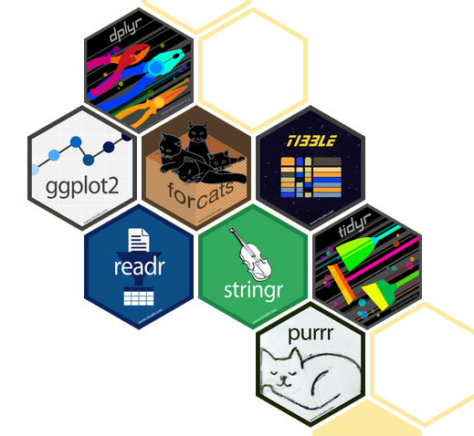
The tidyverse ecosystem

The answer: the tidyverse!

A set of packages developed by RStudio that facilitates:

  • Reading (readr) and manipulating databases (dplyr)
  • Exploiting textual data (stringr), temporal (lubridate) or categorical (forcats)
  • Creating graphics (ggplot2)
  • Programming from dataframes (purrr)
  • And many other things…

The tidy data concept

  • Each variable has its own column;
  • Each observation has its own row;
  • A value, materializing an observation of a variable, is found in a single cell.

Note

Concept popularized by Hadley Wickham.

readr

  • The package for reading flat files (.csv, .txt…)
  • Allows obtaining a tibble, the augmented dataframe of the tidyverse

dplyr

  • The central package of the data manipulation ecosystem;
  • Data manipulation and descriptive statistics;

dplyr

Main verbs

We work on a tibble (augmented dataframe)

  • select(): select variables by their name;
  • rename(): rename variables;
  • filter(): select observations according to one or more conditions;
  • arrange(): sort the table according to one or more variables;
  • mutate(): add variables that are functions of other variables;
  • summarise(): calculate a statistic from data;
  • group_by(): perform operations by group.

dplyr

Data manipulation

The following package(s) will be installed:
- eurostat [4.0.0]
These packages will be installed into "/__w/r-introduction/r-introduction/renv/library/linux-ubuntu-noble/R-4.5/x86_64-pc-linux-gnu".

# Installing packages --------------------------------------------------------
- Installing eurostat 4.0.0 ...                 OK [linked from cache]
Successfully installed 1 package in 5.9 milliseconds.

We chain sequences with pipes (%>%)

library(dplyr)

pop_by_age %>%
1  as_tibble() %>%
2  filter(sex == "F") %>%
3  mutate(x = paste0(age, "_", sex))
1
We convert the standard dataframe to tibble
2
We keep only gas stations (values B316 of TYPEQU)
3
We create a new column by referencing existing ones (without quotes!)


Note

More details in utilitR

dplyr

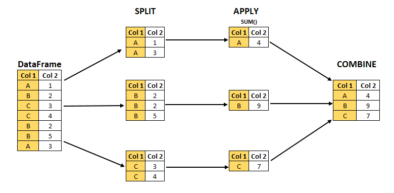
Aggregated statistics

  • split-apply-combine logic with groupby
Illustration of split-apply-combine
library(dplyr)

pop_by_age %>%
1  as_tibble() %>%
2  filter(TIME_PERIOD == "2025-01-01") %>%
3  group_by(geo) %>%
4  summarise(pop_by_country_2025 = sum(values, na.rm = TRUE))
1
We convert the standard dataframe to tibble
2
We keep only gas stations (values 2025-01-01 of TIME_PERIOD)
3
We define geo as a stratification variable to define groups
4
We summarize the data by summing gas stations in each group

ggplot

  • The essential package for making graphics ❤️;
  • Coherent and flexible approach based on the grammar of graphics
    • Subject of a dedicated chapter

stringr, forcats and lubridate

  • Many functions facilitating manipulation:
    • Textual data: stringr
    • Categorical data: forcats
    • Temporal data: lubridate

Data Formats

General Information

  • Data can be stored in many different formats
    • Different standards
    • Different ways of importing
  • Limited functionalities:
    • Specialized packages for certain formats
    • Objective: flatten information into a dataframe

Note

We’ll see geographic formats, and their challenges, later

CSV

  • Flat file format with delimited columns:
    • Standard: , as delimiter, . as decimal;
    • European variant 😮‍💨: ; as delimiter, , as decimal
  • Universal format, simple to use (some limitations)

CSV

  • Reading with the read_csv function from the readr package!
1library(readr)
2read_csv("data_folder/file_name.csv")
1
We import the readr library to have access to the read_csv function
2
We use read_csv to read data stored in the relative path data_folder/file_name.csv

Note

  • CSV with ; delimiter: read_csv2 function.
  • More exotic flat formats (.txt for example): read_delim

More details in the utilitR documentation

JSON

  • The web format, especially for APIs
    • API: we’ll see that later

JSON

  • Imported as a hierarchical list
  • Objective: transform this information into a tidy dataframe
    • Not always easy!
1library(jsonlite)
2df <- fromJSON(file="data_folder/file_name.json")
1
We import the jsonlite library to have access to the fromJSON function
2
We use fromJSON to read data stored in the relative path data_folder/file_name.json

Excel formats

  • Proprietary format

  • Mixes formatting and raw data

    • Not appropriate for data analysis
    • Dangerous for reproducibility and transparency
  • More details on utilitR

The magrittr pipe (%>%)

The magrittr pipe (%>%)

A way to chain operations

library(dplyr)

df <- filter(
  as_tibble(pop_by_age),
  TIME_PERIOD == "2025-01-01"
)

summarise(
  group_by(pop_by_age, geo),
  pop_by_country_2025 = sum(values, na.rm = TRUE)
)
library(dplyr)

pop_by_age %>%
  as_tibble() %>%
  filter(TIME_PERIOD == "2025-01-01") %>% 
  group_by(geo) %>% 
  summarise(pop_by_country_2025 = sum(values, na.rm = TRUE))