Importing and manipulating data with

Check out the slides below or click here to view the slides in full screen.

In this second tutorial, we will learn to import and manipulate data with .

Note

Some code examples include annotations on the side, hover over them to display them, as shown below

"an explanatory annotation accompanies me on the right"

1

I appear when you hover over me 🐭!

In this chapter, we will mainly use the following packages from the tidyverse:

• readr for data import;
• dplyr for data manipulation.

Note

The tidyverse is not the only complete ecosystem for data analysis.

However, for an introduction to , it’s certainly the most reasonable to adopt.

Competing or complementary ecosystems (data.table, arrow, duckdb) already require a good understanding of the tidyverse and its limitations.

In this tutorial, we will use two data sources:

• Greenhouse gas emissions estimated at the municipal level by ADEME. The dataset is available on data.gouv and directly queryable in with this url (this will be the subject of the first exercise)¹.
• Ideally, we would directly use the data available on the Insee website but these require some cleaning work that is beyond the scope of this tutorial. To facilitate importing Insee data, it’s recommended to use the packages doremifasol and insee which simplify access to Insee data available on the insee.fr website or via APIs.

1 Preliminary steps: installing packages

is an open source language. Anyone can therefore propose code to increase the language’s functionalities. A coherent set of functionalities is called a library or package.

Since the team managing the language doesn’t intend to integrate all libraries into the base language (which should remain, as its name indicates, basic), there are community spaces where people can make their packages available. In the ecosystem, the two main ones² are:

• The CRAN (Comprehensive R Archive Network): the official and historical repository of libraries. To install a package stored in this space, use install.package;
• Github : the social network for open source code. To install a package stored in this space, use remotes::install_github³

Note

Generally, packages with certain maturity are on CRAN. Github has a more catch-all aspect where you find gems alongside things of more variable quality.

Some packages we’ll see aren’t on CRAN because the validation procedure to deposit your package there is quite heavy and tiring for volunteer developers, usually unpaid for this work and often doing it at night.

To install a package available on CRAN, for example the dplyr package, you can do:

install.packages("insee")

To install a package available on Github , for example doremifasol which is available on the InseeFrLab account’s repository, do:

remotes::install_github('inseefrlab/DoReMIFaSol')

Here are all the instructions to install the packages needed to perform all the exercises in this tutorial:

install.packages(c("readr","dplyr", "tidyr", "ggplot2", "remotes"))
remotes::install_github('inseefrlab/DoReMIFaSol')

Since we’ll frequently use dplyr, we can import it directly:

library(dplyr)
library(tidyr)
library(stringr)

2 Importing data

2.1 Importing a csv from Ademe

To start, we’ll import Ademe data using the readr package[^readcsv].

Exercise 1: reading a csv with readr and observing the data

Here’s the URL where the data is available

url <- "https://koumoul.com/s/data-fair/api/v1/datasets/igt-pouvoir-de-rechauffement-global/convert"

1. Use the readr package to import this data. Name this object emissions⁴

Solution

library(readr)
emissions <- read_csv(url)

2. Display the first lines with head and observe the display difference with, for example, this dataframe:

df <- data.frame(
  var1 = 1:10,
  var2 = letters[1:10],
  var3 = rep(c(TRUE, FALSE), times = 5)
)

Solution

head(emissions)
head(df)

3. Display the class of emissions. Do you now understand why this object is slightly different from a base dataframe?

Solution

class(emissions)

4. Use appropriate functions for the first 10 values, the last 15 and a random sample of 10 values using the appropriate function from the dplyr package

If stuck on question 1

Read the read_csv documentation (very well done) or search for examples online to discover this function. ⚠️ Don’t use read.csv (base function) which isn’t performant.

2.2 First data manipulations

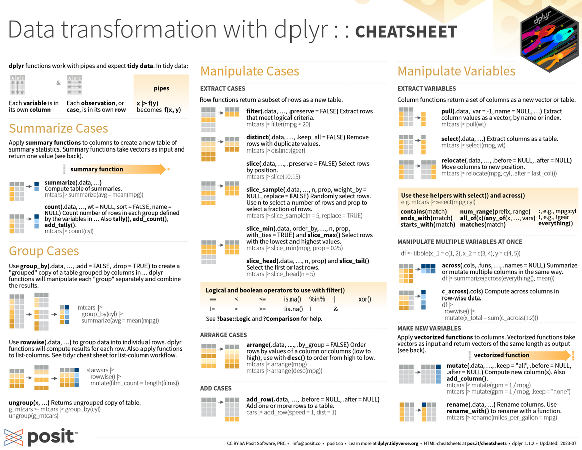
As mentioned in utilitR, the main functions of dplyr (the verbs of the dplyr grammar) are as follows:

• select(): select variables by their name;
• rename(): rename variables;
• filter(): select observations according to one or more conditions;
• arrange(): sort the table according to one or more variables;
• mutate(): add variables that are functions of other variables;
• summarise(): calculate a statistic from data;
• group_by(): perform operations by group.

viewof dplyrVerbs = Inputs.select(['select','rename','filter','mutate', 'arrange'], {value: "select"})

html`<img src="https://github.com/linogaliana/r-geographie/raw/main/exercises/img/${dplyrVerbs}.png" width="60%"</>`

Figure 1: Illustration of dplyr verbs

The following cheatsheet is very practical as it illustrates these different functions. It’s recommended to regularly consult it (click on the image to zoom 🔎):

dplyr Cheatsheets

Exercise 2: discovering dplyr verbs for data manipulation

First, let’s familiarize ourselves with operations on columns.

1. Create a dataframe emissions_copy keeping only the columns INSEE commune, Commune, Autres transports and Autres transports international

Hint for this question

2. Since variable names are impractical, rename them as follows:
   • INSEE commune \(\to\) code_insee
   • Autres transports \(\to\) transports
   • Autres transports international \(\to\) transports_international

Hint for this question

3. To simplify, let’s replace missing values (NA) with the value 0⁵. Use the replace_na function from the tidyr package, in conjunction with mutate, to transform missing values to 0.

Hint for this question

4. Create the following variables in the same code sequence:
   • dep: the department. This can be created using the first two characters of code_insee with the str_sub function from the stringr package⁶
   • transports_total: transport sector emissions (sum of the two variables)

Hint for this question

5. Order the data from highest to lowest polluter then order the data from highest to lowest polluter by department (from 01 to 95).

Hint for this question

6. Calculate total emissions by department

Hint for this question

• “Group by” = group_by
• “total emissions” = summarise(sum(***))

Solution question 1

emissions_copy <- emissions %>%
  select(`INSEE commune`, `Commune`, `Autres transports`, `Autres transports international`)

Solution question 2

emissions_copy <- emissions_copy %>%
  rename(
    code_insee = `INSEE commune`,
    transports = `Autres transports`,
    transports_international = `Autres transports international`
    )

Solution question 3

emissions_copy <- emissions_copy %>%
  mutate(
    transports = replace_na(transports),
    transports_international = replace_na(transports_international)
    )

Solution question 4

emissions_copy <- emissions_copy %>%
  mutate(
    dep = str_sub(code_insee, 1, 2),
    transports_total = transports + transports_international
    )

Solution question 5

emissions_copy %>%
  arrange(desc(transports_total))

emissions_copy %>%
  arrange(dep, desc(transports_total))

Solution question 6

emissions_copy %>%
  group_by(dep) %>%
  summarise(sum(transports_total))

2.3 Importing Insee data

For our municipal information, we’ll use one of Insee’s most used sources: Filosofi data. To facilitate retrieving these, we’ll use the community package doremifasol:

library(doremifasol)
library(tibble)
filosofi <- as_tibble(
  telechargerDonnees("FILOSOFI_COM", date = 2016)
)
head(filosofi)

# A tibble: 6 × 29
  CODGEO LIBGEO      NBMENFISC16 NBPERSMENFISC16  MED16 PIMP16 TP6016 TP60AGE116
  <chr>  <chr>             <dbl>           <dbl>  <dbl>  <dbl>  <dbl>      <dbl>
1 01001  L'Abergeme…         313            796. 22679      NA     NA         NA
2 01002  L'Abergeme…         101            248  24382.     NA     NA         NA
3 01004  Ambérieu-e…        6363          14228  19721      49     17         19
4 01005  Ambérieux-…         633           1662. 23378      NA     NA         NA
5 01006  Ambléon              NA             NA     NA      NA     NA         NA
6 01007  Ambronay           1087           2684  22146.     57     NA         NA
# ℹ 21 more variables: TP60AGE216 <dbl>, TP60AGE316 <dbl>, TP60AGE416 <dbl>,
#   TP60AGE516 <dbl>, TP60AGE616 <dbl>, TP60TOL116 <dbl>, TP60TOL216 <dbl>,
#   PACT16 <dbl>, PTSA16 <dbl>, PCHO16 <dbl>, PBEN16 <dbl>, PPEN16 <dbl>,
#   PPAT16 <dbl>, PPSOC16 <dbl>, PPFAM16 <dbl>, PPMINI16 <dbl>, PPLOGT16 <dbl>,
#   PIMPOT16 <dbl>, D116 <dbl>, D916 <dbl>, RD16 <dbl>

Note

The as_tibble function converts the base dataframe (doremifasol doesn’t make assumptions about the manipulation ecosystem adopted) into a dataframe adapted for use via the tidyverse.

3 Data cleaning

Exercise 2

Since readr or doremifasol automatically handled the data import, let’s do a small quality control:

1. Display the column names of our dataframes emissions and filosofi. What are the common columns? Use the intersect function and understand the nature of the problem.
2. Observe the structure of our datasets (column types). Are the default types appropriate?

Then, we verify the dimensions of the DataFrames and the structure of some key variables. In this case, the fundamental variables for linking our data are the municipal variables. Here, we have two geographic variables: a municipality code and a municipality name. We’ll therefore verify they’re well suited for statistical analysis.

3. Check the dimensions of the dataframes;
4. Check the number of unique values of geographic variables in each base. Do the results appear consistent?
5. Identify in filosofi the municipality names that correspond to multiple municipality codes and select their codes. In other words, identify the CODGEO such that there are duplicate LIBGEO and store them in a dataframe duplicates

We temporarily focus on observations where the label has more than two different municipality codes

6. Look at these observations in filosofi. For better visibility, reorder the obtained base alphabetically
7. Determine the average size (variable number of people: NBPERSMENFISC16) and some descriptive statistics of this data. Compare to the same statistics on data where labels and municipality codes coincide
8. Check large cities (more than 100,000 people), the proportion of cities for which the same name is associated with different municipality codes.
9. Check in filosofi the cities whose label equals Montreuil. Also check those containing the term ‘Saint-Denis’

Solution question 1

str(emissions)
intersect(colnames(filosofi), colnames(emissions))

Solution question 2

str(filosofi)
str(emissions)

Solution question 3

dim(filosofi)
dim(emissions)

Solution question 3

emissions %>%
  select('INSEE commune', 'Commune') %>%
  summarize(Unique_Count = n_distinct(Commune))

filosofi %>%
  select('CODGEO', 'LIBGEO') %>%
  summarize(Unique_Count = n_distinct(LIBGEO))

Solution questions 5 to 7

# Question 5
duplicates <- filosofi %>%
  group_by(LIBGEO) %>%
  summarize(Count = n()) %>%
  select(LIBGEO, Count) %>%
  #arrange(desc(Count)) %>%
  filter(Count > 1)

# Question 6
filosofi %>%
  filter(LIBGEO %in% duplicates$LIBGEO) %>%
  arrange(LIBGEO)

# Question 7
filosofi %>%
  filter(LIBGEO %in% duplicates$LIBGEO) %>%
  summarize(Stats = mean(NBPERSMENFISC16, na.rm = TRUE))

# Calculate summary statistics for 'NBPERSMENFISC16' for rows where 'LIBGEO' is not in 'x$LIBGEO'
filosofi %>%
  filter(!(LIBGEO %in% duplicates$LIBGEO)) %>%
  summarize(Stats = mean(NBPERSMENFISC16, na.rm = TRUE))

Solution question 8

filosofi_big <- filosofi %>%
  filter(NBPERSMENFISC16 > 100000) %>%
  mutate(probleme = LIBGEO %in% duplicates$LIBGEO)

# Proportion of problematic cities
mean_probleme <- filosofi_big %>%
  summarize(mean(probleme))

# Filter rows where 'probleme' is TRUE
df_probleme <- filosofi_big %>%
  filter(probleme)

What you should find in questions 8 and 9

For question 8, you should get this:

head(df_probleme)

# A tibble: 4 × 30
  CODGEO LIBGEO      NBMENFISC16 NBPERSMENFISC16  MED16 PIMP16 TP6016 TP60AGE116
  <chr>  <chr>             <dbl>           <dbl>  <dbl>  <dbl>  <dbl>      <dbl>
1 93048  Montreuil         43996         108682  18428      55     26         29
2 93066  Saint-Denis       39469         108346. 14622.     39     38         35
3 97411  Saint-Denis       57567         145396. 16317.     35     34         47
4 97415  Saint-Paul        37064         105829  16279.     35     33         42
# ℹ 22 more variables: TP60AGE216 <dbl>, TP60AGE316 <dbl>, TP60AGE416 <dbl>,
#   TP60AGE516 <dbl>, TP60AGE616 <dbl>, TP60TOL116 <dbl>, TP60TOL216 <dbl>,
#   PACT16 <dbl>, PTSA16 <dbl>, PCHO16 <dbl>, PBEN16 <dbl>, PPEN16 <dbl>,
#   PPAT16 <dbl>, PPSOC16 <dbl>, PPFAM16 <dbl>, PPMINI16 <dbl>, PPLOGT16 <dbl>,
#   PIMPOT16 <dbl>, D116 <dbl>, D916 <dbl>, RD16 <dbl>, probleme <lgl>

While for question 9, your two dataframes will look like

Solution question 9

# Question 9
filosofi %>%
  filter(LIBGEO == 'Montreuil')

# A tibble: 4 × 29
  CODGEO LIBGEO    NBMENFISC16 NBPERSMENFISC16  MED16 PIMP16 TP6016 TP60AGE116
  <chr>  <chr>           <dbl>           <dbl>  <dbl>  <dbl>  <dbl>      <dbl>
1 28267  Montreuil         215            503  24823.     NA     NA         NA
2 62588  Montreuil         994           1951  18762      NA     NA         NA
3 85148  Montreuil         340            884. 19340      NA     NA         NA
4 93048  Montreuil       43996         108682  18428      55     26         29
# ℹ 21 more variables: TP60AGE216 <dbl>, TP60AGE316 <dbl>, TP60AGE416 <dbl>,
#   TP60AGE516 <dbl>, TP60AGE616 <dbl>, TP60TOL116 <dbl>, TP60TOL216 <dbl>,
#   PACT16 <dbl>, PTSA16 <dbl>, PCHO16 <dbl>, PBEN16 <dbl>, PPEN16 <dbl>,
#   PPAT16 <dbl>, PPSOC16 <dbl>, PPFAM16 <dbl>, PPMINI16 <dbl>, PPLOGT16 <dbl>,
#   PIMPOT16 <dbl>, D116 <dbl>, D916 <dbl>, RD16 <dbl>

Solution question 9

# Question 10
filosofi %>%
  filter(grepl('Saint-Denis', LIBGEO)) %>%
  head(10)

# A tibble: 10 × 29
   CODGEO LIBGEO     NBMENFISC16 NBPERSMENFISC16  MED16 PIMP16 TP6016 TP60AGE116
   <chr>  <chr>            <dbl>           <dbl>  <dbl>  <dbl>  <dbl>      <dbl>
 1 01344  Saint-Den…        2562           6036  23258      63      7         NA
 2 01345  Saint-Den…         965           2280  21464      53     NA         NA
 3 02818  Villiers-…         365            901  22221      NA     NA         NA
 4 11339  Saint-Den…         224            474. 18477.     NA     NA         NA
 5 14571  Saint-Den…         124            298. 20860.     NA     NA         NA
 6 14572  Saint-Den…         331            770. 20080      NA     NA         NA
 7 17323  Saint-Den…         733           1401  21364.     NA     NA         NA
 8 18204  Saint-Den…         125            314. 21446.     NA     NA         NA
 9 21442  Morey-Sai…         285            664. 25946.     NA     NA         NA
10 25129  Chassagne…          50            116  21357.     NA     NA         NA
# ℹ 21 more variables: TP60AGE216 <dbl>, TP60AGE316 <dbl>, TP60AGE416 <dbl>,
#   TP60AGE516 <dbl>, TP60AGE616 <dbl>, TP60TOL116 <dbl>, TP60TOL216 <dbl>,
#   PACT16 <dbl>, PTSA16 <dbl>, PCHO16 <dbl>, PBEN16 <dbl>, PPEN16 <dbl>,
#   PPAT16 <dbl>, PPSOC16 <dbl>, PPFAM16 <dbl>, PPMINI16 <dbl>, PPLOGT16 <dbl>,
#   PIMPOT16 <dbl>, D116 <dbl>, D916 <dbl>, RD16 <dbl>

This small exercise is reassuring because the duplicate labels are actually identical municipality names that aren’t in the same department. These aren’t duplicate observations. We’ll therefore rely on municipality codes, which are unique.

Exercise 3

Let’s start data exploration. This involves some data cleaning beforehand.

1. Rename the variable INSEE commune to code_insee⁷.
2. The first two digits of municipality codes are the department number. Create a department variable dep in emissions and in filosofi using the str_sub function from the stringr package⁸.

Let’s start calculating our first descriptive statistics.

3. Calculate total emissions by sector for each department. Log-transform these results in an object emissions_log. Figure 2 illustrates the structure of these emissions for 5 random departments.

4. Start from the emissions dataset. Calculate total emissions by department and output the list of the top 10 CO2 emitters and the 5 lowest-emitting departments. Without doing a merge, look at the characteristics of these departments (population and standard of living)

Solution question 1

library(stringr)

emissions <- emissions %>%
  rename('code_insee' = `INSEE commune`)

Solution question 2

emissions <- emissions %>%
  mutate(dep = str_sub(code_insee, start = 1, end = 2))
filosofi <- filosofi %>%
  mutate(dep = str_sub(CODGEO, start = 1, end = 2))

Solution question 3

emissions_log <- emissions %>%
    group_by(dep) %>%
    summarise(across(where(is.numeric), sum, na.rm = TRUE)) %>%
    mutate(across(where(is.numeric), log))

Solution question 4

## Total emissions by department
emissions_dep <- emissions %>%
  mutate(total = rowSums(pick(where(is.numeric)), na.rm = TRUE)) %>%
  group_by(dep) %>%
  summarise(total = sum(total))
gros_emetteurs <- emissions_dep %>%
  arrange(desc(total)) %>%
  head(10)
petits_emetteurs <- emissions_dep %>%
  arrange(total) %>%
  head(5)

## Characteristics of these departments in filosofi
gros_emetteurs_filosofi <- filosofi %>%
  filter(dep %in% gros_emetteurs$dep) %>%
  group_by(dep) %>%
  summarise(across(c('NBPERSMENFISC16','MED16'), \(x) mean(x, na.rm = TRUE)))

head(gros_emetteurs_filosofi)

Code to create the figure below

library(tidyr)
library(ggplot2)

emissions_log_sample <- emissions_log %>%
  filter(dep %in% sample(unique(dep),5))

emissions_log_sample <- emissions_log_sample %>%
  pivot_longer(cols = -dep, names_to = "Category", values_to = "Value")

ggplot(emissions_log_sample, aes(x = dep, y = Value, fill = Category)) +
    geom_bar(stat = "identity") +
    labs(x = "Department", y = "Value") +
    theme_minimal() +
    theme(axis.text.x = element_text(angle = 45, hjust = 1)) + scale_fill_viridis_d()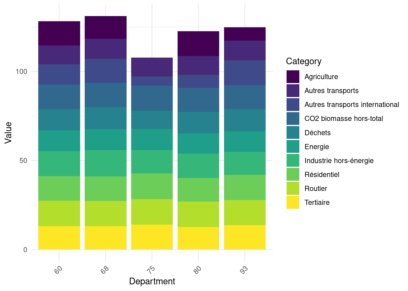

Figure 2: Emission structure of five random departments

Example of using str_sub

library(stringr)
df %>% mutate(x = str_sub(y, start = 3, end = 5))

4 Restructuring data

Two types of data are generally presented:

• wide format: data contains repeated observations for the same individual (or group) in different columns
• long format: data contains repeated observations for the same individual in different rows with a column to distinguish observation levels

An example of the distinction between the two can be taken from Hadley Wickham’s reference work, R for Data Science:

Long (left) and wide (right) data (source: R for Data Science)

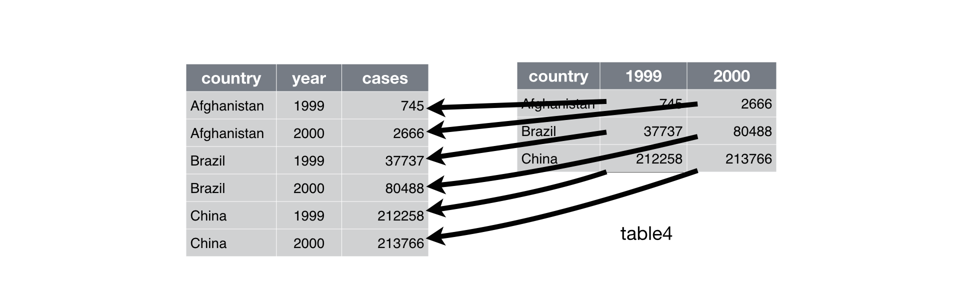
We often need to restructure data with to lengthen them (wide to long) and widen them (long to wide). The tidyr package (which belongs to the tidyverse) allows these types of transformations.

The following cheat sheet will help remember which functions to apply if needed:

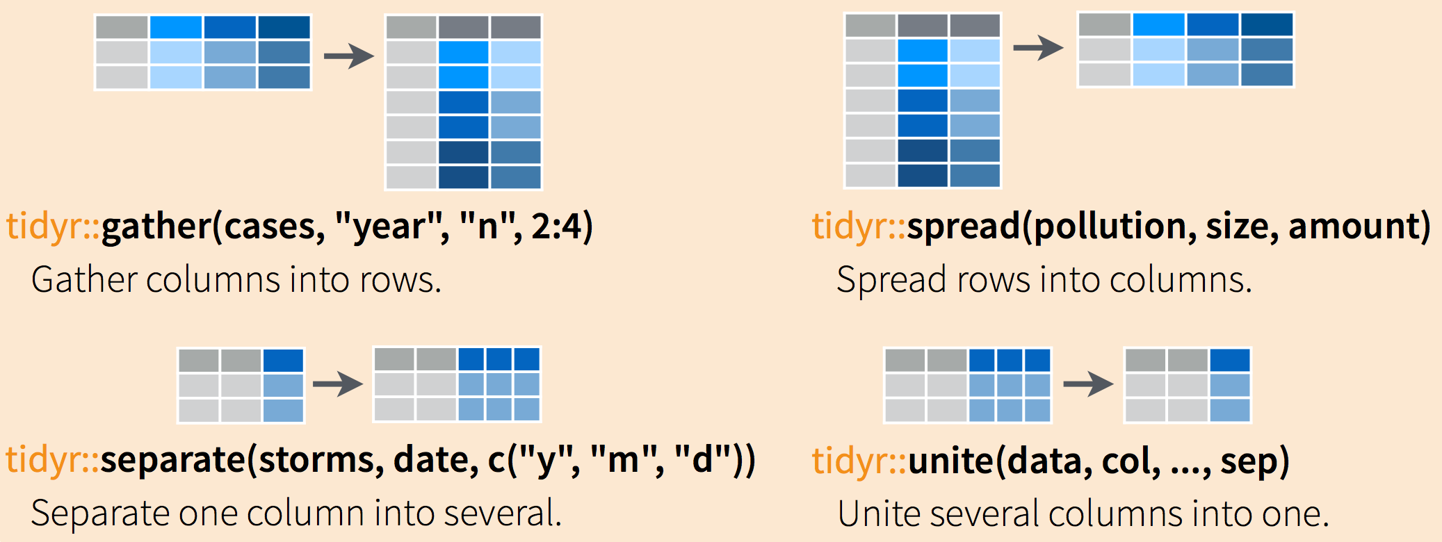
Going from wide to long format (or vice-versa) can be extremely practical because certain functions are more suitable for one data form or another.

Generally, long formats are often preferable because it’s easier to iterate over rows than columns due to ’s vectorial nature. This is particularly the preferred data form for preparing graphs with ggplot, which we’ll discover in the next chapter.

Exercise 4: the wide to long transformation

1. Restructure the data to long format to have emissions data by sector while keeping the municipality as the analysis level (be careful with other identifying variables).
2. Sum by sector and graphically represent a barplot⁹
3. Keep, for each department, the most polluting sector

Solution question 1

library(tidyr)

df_long <- emissions %>%
  pivot_longer(cols = -c(code_insee, Commune, dep),
               names_to = "secteur",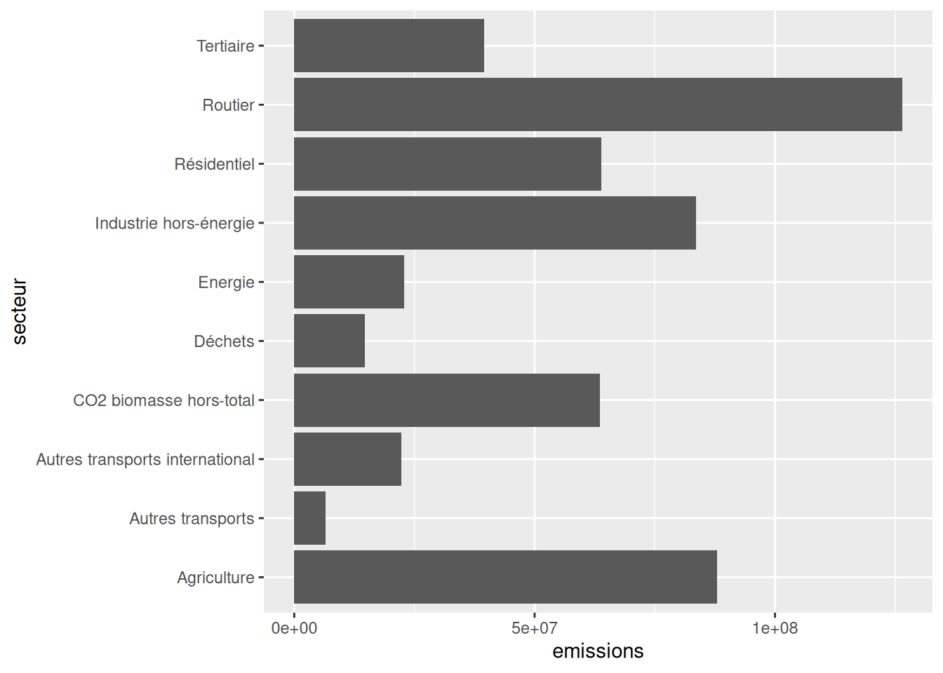
               values_to = "emissions")

Solution question 2

df_long_summary <- df_long %>%
  group_by(secteur) %>% summarise(emissions = sum(emissions, na.rm = TRUE))

Graph to create for question 2

Once the df_long_summary dataframe is created, the minimal code to create the desired barplot is:

ggplot(df_long_summary) +
  geom_bar(
    aes(y = secteur, x = emissions),
    stat ='identity'
  )

No need to go further for now, we’ll do more ggplot later.

Solution question 3

df_long_dep <- df_long %>%
  group_by(secteur, dep) %>%
  summarise(emissions = sum(emissions, na.rm = TRUE)) %>%
  arrange(desc(dep), desc(emissions)) %>%
  group_by(dep) %>%
  slice_head(n = 1)

# A tibble: 6 × 3
# Groups:   dep [6]
  secteur     dep   emissions
  <chr>       <chr>     <dbl>
1 Routier     01     1635350.
2 Routier     02     1386403.
3 Agriculture 03     1949985.
4 Routier     04      390568.
5 Routier     05      345859.
6 Routier     06     1561664.

Exercise 5: long to wide

TO DO

5 Combining data

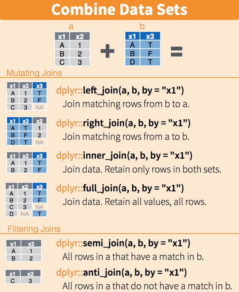
Information we seek is increasingly obtained from multiple data sources rather than a single database. It’s becoming common to need to combine data from different sources.

We’ll focus here on the most favorable case which is when information allows exact matching of two databases (otherwise we’d be in a much more complex situation of fuzzy matching). The typical situation is matching between two data sources using an individual identifier or municipality code identifier, which is our case.

It’s recommended to read this fairly complete guide on joins with which also gives useful recommendations for Python .

In common statistical language, the terms merge or join are used interchangeably. The second term comes from SQL syntax and is the one rather used when coding with dplyr.

The different types of join available in dplyr

Exercise 6: enriching emissions data

First, we’ll calculate each municipality’s carbon footprint.

1. Calculate total emissions using the following command (since this is complex, we give it directly):

emissions <- emissions %>%
  mutate(total = rowSums(pick(where(is.numeric)), na.rm = TRUE))

2. Perform a left join between emissions data and framing data¹⁰.

3. Calculate carbon footprint (total emissions / population).

At this stage we might want to move toward modeling to try to explain carbon footprint determinants from municipal variables. However, an inferential approach requires checking descriptive statistics beforehand to be relevant.

4. Use the following code to output a histogram in level then in log of municipal carbon footprint;

ggplot(emissions_merged) +
  geom_histogram(aes(x = empreinte, y = after_stat(density))) +
  scale_x_log10()

5. For each city, compare carbon footprint to the department median. In relative terms, which cities are particularly virtuous (i.e., those with emissions well below the department average)?

With better understanding of our data, we’re approaching inferential statistics. However, we’ve so far built univariate statistics but haven’t sought to understand results by looking at the link with other variables. This brings us to bivariate statistics, particularly correlation analysis. This work is important since any subsequent modeling will consist of refining correlation analysis to account for cross-correlations between multiple factors. We propose here to do this analysis in a minimal way.

6. Look at the correlation between framing variables and carbon footprint (the solution is given, as the manipulations aren’t obvious). Do some variables seem to potentially influence carbon footprint?

Solution question 1

emissions <- emissions %>%
  mutate(total = rowSums(pick(where(is.numeric)), na.rm = TRUE))

Solution question 2

emissions_merged <- emissions %>%
  left_join(filosofi, by = c("code_insee" = "CODGEO"))

Solution question 3

emissions_merged <- emissions_merged %>%
  mutate(empreinte = total/NBPERSMENFISC16)

Solution question 4

ggplot(emissions_merged) +
  geom_histogram(aes(x = empreinte, y = after_stat(density))) +
  scale_x_log10()

Solution question 5

emissions_merged <- emissions_merged %>%
  rename(departement = dep.x) %>%
  group_by(departement) %>%
  mutate(empreinte_mediane = median(empreinte, na.rm = TRUE)) %>%
  mutate(empreinte_relative = empreinte/empreinte_mediane)

emissions_merged %>% arrange(empreinte_relative)

Solution question 6

library(tibble)

correlations <- cor(
  emissions_merged %>% ungroup() %>% select(where(is.numeric)),
  use="complete.obs"
  )[,'empreinte']

correlations <- enframe(correlations) %>%
  filter(name %in% colnames(filosofi)) %>%
  arrange(desc(abs(value)))

Here’s a quick visualization of correlations with carbon footprint:

ggplot(correlations) + geom_bar(aes(x = value, y = name), stat = "identity") +
  scale_y_discrete(limits = correlations$name)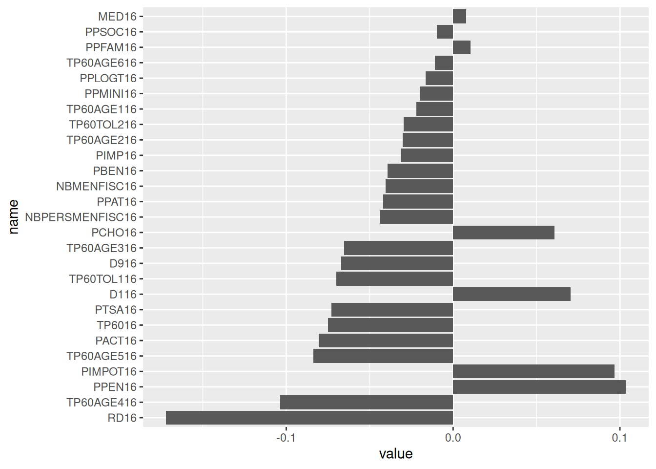 

6 Corrections

You can find all corrections here.

Footnotes

1. readr offers the possibility to import data directly from a url. This is the option taken in this tutorial. If you prefer, for network access or performance reasons, to import from a local machine, you can download the data and change the import commands with the appropriate path instead of the url.

2. There’s also bioconductor but since it’s mainly oriented towards biostatistics (one of the academic communities that adopted earliest), we don’t really use it

3. remotes::install_github means to use the install_github function from the package remotes. In other words, you need a package to install other packages 🤯. This is because Github didn’t exist when was created (1990s) and this functionality hasn’t been added since.

4. For lack of imagination, we’re often tempted to call our main dataframe df or data. This is often a bad idea since this name isn’t very informative when rereading the code a few weeks later. Self-documentation, an approach that consists of having code that explains itself, is a good practice and it’s therefore recommended to give a simple but effective name to know the nature of the dataset in question.

5. This assumption is certainly false. It’s exclusively here to illustrate variable creation via mutate.

6. To be really precise, we would need to modify the values obtained for Corsican departments with the case_when function from the dplyr package. This is left as an additional exercise.

7. The space in the variable name is annoying. To be able to use this variable’s name in rename, we’ll need to use backticks, i.e., INSEE commune.

8. The limited functionalities of the base language for text manipulation quickly become constraining. We thus quickly move to stringr even though it’s not the main subject of the chapter.

9. you can directly use the helper code snippet if you’re not familiar with ggplot

10. Ideally, we should ensure this join doesn’t introduce bias. Indeed, since our reference years aren’t necessarily identical, there may be a mismatch between our two sources. Since the tutorial is already long, we won’t go down this path. Interested readers can perform such an analysis as an additional exercise.